Fit of the coefficients
- class mrestimator.FitResult(tau, mre, fitfunc, taustderr=None, mrestderr=None, tauquantiles=None, mrequantiles=None, quantiles=None, popt=None, pcov=None, ssres=None, rsquared=None, steps=None, dt=1, dtunit='ms', desc=None, description=None)[source]
Result returned by fit(). Subclassed from
namedtuple.- Variables:
tau (float) – The estimated autocorrelation time in dtunits. Default is ‘ms’.
mre (float) – The branching parameter estimated from the multistep regression.
fitfunc (callable) – The model function, f(x, …). This allows to fit directly with popt. To get the (TeX) description of a (builtin) function, use
ut.math_from_doc(fitfunc).popt (array) – Final fitparameters obtained from the (best) underlying
scipy.optimize.curve_fit(). Beware that these are not corrected for the time bin size, this needs to be done manually (for time and frequency variables).pcov (array) – Final covariance matrix obtained from the (best) underlying
scipy.optimize.curve_fit().ssres (float) – Sum of the squared residuals for the fit with popt. This is not yet normalised per degree of freedom.
steps (array) – The step numbers \(k\) of the coefficients \(r_k\) that were included in the fit. Think fitrange.
dt (float) – The size of each step in dtunits. Default is 1.
dtunit (str) – Units of step size and the calculated autocorrelation time. Default is ‘ms’. dt and dtunit are inherited from
CoefficientResult. Overwrite by providing data fromcoefficients()and the desired values set there.quantiles (list or None) – Quantile values (between 0 and 1, inclusive) calculated from bootstrapping. See
numpy.quantile. Defaults are[.125, .25, .4, .5, .6, .75, .875]tauquantiles (list or None) – Resulting \(\tau\) values for the respective quantiles above.
mrequantiles (list or None) – Resulting \(m\) values for the respective quantiles above.
description (str) – Description, inherited from
CoefficientResult. description provided tofit()takes priority, if set.
Example
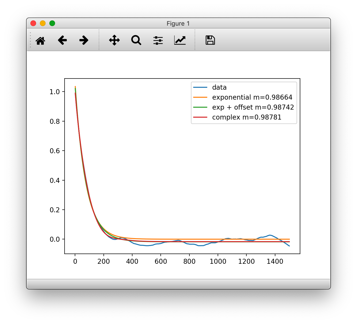
import numpy as np
import matplotlib.pyplot as plt
import mrestimator as mre

bp = mre.simulate_branching(m=0.99, a=10, numtrials=15)
rk = mre.coefficients(bp, dtunit='step')

# compare the builtin fitfunctions
m1 = mre.fit(rk, fitfunc=mre.f_exponential)
m2 = mre.fit(rk, fitfunc=mre.f_exponential_offset)
m3 = mre.fit(rk, fitfunc=mre.f_complex)

# plot manually without using OutputHandler
plt.plot(rk.steps, rk.coefficients, label='data')
plt.plot(rk.steps, mre.f_exponential(rk.steps, *m1.popt),
    label='exponential m={:.5f}'.format(m1.mre))
plt.plot(rk.steps, mre.f_exponential_offset(rk.steps, *m2.popt),
    label='exp + offset m={:.5f}'.format(m2.mre))
plt.plot(rk.steps, mre.f_complex(rk.steps, *m3.popt),
    label='complex m={:.5f}'.format(m3.mre))

plt.legend()
plt.show()
- mrestimator.fit(data, fitfunc=<function f_exponential_offset>, steps=None, fitpars=None, fitbnds=None, maxfev=None, ignoreweights=True, numboot=0, quantiles=None, seed=101, desc=None, description=None)[source]
Estimate the Multistep Regression Estimator by fitting the provided correlation coefficients \(r_k\). The fit is performed using
scipy.optimize.curve_fit()and can optionally be provided with (multiple) starting fitparameters and bounds.- Parameters:
data (CoefficientResult or array) – Correlation coefficients to fit. Ideally, provide this as
CoefficientResultas obtained fromcoefficients(). If arrays are provided, the function tries to match the data.fitfunc (callable, optional) – The model function, f(x, …). Directly passed to curve_fit(): It must take the independent variable as the first argument and the parameters to fit as separate remaining arguments. Default is
f_exponential_offset. Other builtin options aref_exponentialandf_complex.steps (array, optional) – Specify the steps \(k\) for which to fit (think fitrange). If an array of length two is provided, e.g.
steps=(minstep, maxstep), all enclosed values present in the provdied data, including minstep and maxstep will be used. Arrays larger than two are assumed to contain a manual choice of steps and those that are also present in data will be used. Strides other than one are possible. Ignored if data is not passed as CoefficientResult. Default: all values given in data are included in the fit.fitpars (ndarray, optional) – The starting parameters for the fit. If the provided array is two dimensional, multiple fits are performed and the one with the smallest sum of squares of residuals is returned.
fitbounds (ndarray, optional) – Lower and upper bounds for each parameter handed to the fitting routine. Provide as numpy array of the form
[[lowpar1, lowpar2, ...], [uppar1, uppar2, ...]]numboot (int, optional) – Number of bootstrap samples to compute errors from. Default is 0
seed (int, None or 'random', optional) – If numboot is not zero, provide a seed for the random number generator. If
seed=None, seeding will be skipped. Per default, the rng is (re)seeded everytime fit() is called so that every repeated call returns the same error estimates.quantiles (list, optional) – If numboot is not zero, provide the quantiles to return (between 0 and 1). See
numpy.quantile. Defaults are[.125, .25, .4, .5, .6, .75, .875]maxfev (int, optional) – Maximum iterations for the fit.
description (str, optional) – Provide a custom description.
- Returns:
FitResult– The output is grouped and can be accessed using its attributes (listed below).